This article explains what affects performance in AudioNodes, and gives you some tips to monitor and improve it in your projects.
Performance Overview
As with all digital audio workstations, you’ll eventually run into a performance ceiling as you keep adding increasingly complex logic into your project. This is especially easy to do in AudioNodes, because everything is modular, and modules (or Nodes) can pile up quick.
When you run into the performance ceiling, buffer underrun occurs, causing audible glitching. It’s when you hear your audio output to be crackling and stuttering.
Performance in AudioNodes depends on 2 factors:
- Nodes you use, and your patch in general — the more Nodes you use (or more complex Nodes you use), the worse performance gets
- Your machine — the faster your machine, the more Nodes you can use before performance degrades
Performance Optimization Tips
An important rule of thumb with optimization is measuring results. To help you with that, AudioNodes has a processing load meter, shown at the top as a percentage (see the Processing Load % section below). Keep an eye on its value to see how your project is performing after a specific change.
The rest of this section gives you some tips to reduce your processing load.
Leverage Constant Folding
AudioNodes has an automatic, powerful optimization process called Constant Folding, which enables Nodes to run in constant mode if certain conditions are met. A Node running in constant mode has zero performance impact, and can be used in large numbers without any performance problems whatsoever.
While you don’t have to do anything for it to work, some patches work better for constant folding, some don’t. Check out the article to learn how you can maximize its impact to improve performance.
Avoid Too Many Expensive Nodes
Different Nodes can have wildly different performance characteristics. A Gain Node, for example, is basically free and even several thousand won’t make a real dent in performance.
On the other hand, the following Nodes, for example, are particularly expensive:
- Pitch Shift Node — large resolution settings are very expensive
- Poly Subpatch Node — a large number of voices can get expensive fast, especially if the internal patch is complex
- Convolver Node — a large room setting with a high reflection %, or an otherwise long impulse response is expensive
If you can, minimize the usage of expensive Nodes, or use a cheaper configuration setup for them. A few tips as a rule of thumb with Nodes:
- Each Node has a performance impact on its own. That is, 2 Convolver Nodes with the same configuration have 2x as much performance impact as 1.
- A common pitfall is having multiple lines of audio, and using the same Convolver Node configuration (or other expensive effect processing) on each of them, one by one. Instead, try to first mix your audio together, and then use a single Convolver Node at the end, if possible.
- You can easily delete multiple Nodes, and then undo the deletion using Ctrl/Cmd + Z (as long as you keep AudioNodes open). This is a quick and easy way to identify which part of your patch is causing the most load. Keep an eye on whether processing load drops significantly after deleting some Nodes, or not.
Freeze Nodes
A powerful feature of AudioNodes is the ability to freeze Nodes in a subpatch, using the Rendered Subpatch Node. This process is the equivalent of freezing a track in other DAWs.
Nodes inside a Rendered Subpatch Node’s subpatch are rendered into an optimized output, and don’t contribute to processing load once the optimized output is rendered.
See Freezing Nodes & Tracks for more details.
Reduce Sample Rate
This comes at a loss of audio fidelity during real-time playback, but you can reduce the global sample rate used in AudioNodes in settings (from the top left corner). Using a sample rate of 22k is twice as fast as using a sample rate of 44.1k, for example.
You can still export high quality renders just the same, while your real-time playback is now much cheaper.
Group Nodes Visually into Subpatches
AudioNodes has a lot of real-time visualization to tell you what’s happening. The most obvious example is connections flashing as a signal goes through them, but Nodes in the Analyzers category also belong here.
This kind of visualization has some additional processing cost. While the performance impact of this is generally negligible compared to the actual processing done by Nodes, it still comes with some performance overhead.
However, Nodes that are not visible on the current patch (i.e. Nodes inside subpatches, while you are on the main patch) don’t process visualization, and thus don’t have any extra overhead. This can sometimes help with performance, even if just a tiny bit.
Close Other Apps & Tabs
This probably goes without saying, and is probably the first thing you find in those low quality AI generated articles on the web, but your machine shares your available CPU capacity between what you have open (including processes running in the background).
Those other processes can take up CPU cycles, and ultimately cause AudioNodes to run out of processing capacity earlier than what your machine could otherwise handle. Thus, it’s a good idea to close them if you run into performance issues. Same goes for browser tabs, especially with the AudioNodes web app.
Processing Load %
AudioNodes displays a processing load monitor in the header. This is a percentage value displaying how much real-time processing power your current project is using:
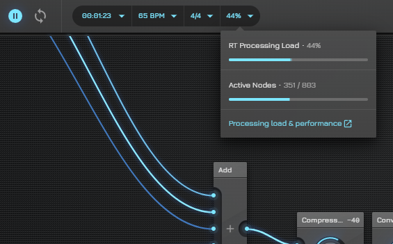
RT Processing Load
This number indicates the total processing load used in the real-time audio thread in AudioNodes. There is only one real-time audio thread in AudioNodes. Every single Node that’s not in either constant mode, or a frozen subpatch, contributes to this number (to varying degrees).
So, the lower the number, the better:
- 0% means AudioNodes is basically idle
- 40-60% means AudioNodes is using half of what your machine can do, and has some more headroom for additional Nodes still — this is a safe, optimal load, where you are using enough of your machine’s capabilities, but you are typically safe from glitching
- 80% (or up) means you are very close to your machine’s limits; in practice, glitching is imminent at these levels (with varying frequency) — at this load level, you’ll typically want to look into optimizing your project
- 100% (MAX) means your machine is working at capacity, and is unable to process your project; audio is skipped and audible glitching occurs — at this level, you need to optimize your project somehow
Note: While the processing load meter should be pretty accurate, there is one thing to keep in mind. Currently, orphaned Nodes (= Nodes not ultimately connected to an Audio Destination Node) that just output into nothing are not always correctly measured. As a result, with a project with a lot of Nodes not connecting to anything, the meter may display a lower-than-actual processing load.
Active Nodes
This indicates the number of Nodes in your project that actively contribute to the real-time processing load. The number also includes Nodes from Subpatch Nodes (including the internal patch of custom Nodes), as well as Nodes from additional Poly Subpatch Node voices. For this reason, it might show a much higher number than what you see on your main patch.
It’s common for interesting, complex projects to have more than 1000 Nodes shown here.
A Node is not considered active when it’s free and doesn’t contribute to processing load. This happens when either:
- It has nothing to do with signal processing (most melody Nodes, Comment Node, etc.)
- It’s running in constant mode, or
- It’s in a Rendered Subpatch Node that’s frozen
Performance When Exporting Projects
Performance when exporting projects is secondary, because it’s not a real-time process, and a high processing load won’t cause glitching. In a way, you can say that the export process is always using a 100% processing load, and is speeding up or slowing down accordingly.
However, the more expensive your project, the longer it will take for the export process to complete. This is typically closely correlated to real-time processing load: a project with a 50% processing load will take roughly twice as long to export as a project with a 25% processing load (assuming they have the same duration, and you use the same export settings).